
Videos
Employ the multiple-application Simpson's rule to evaluate the vertical distance traveled by a rocket if the vertical velocity is given by
In addition, use numerical
To calculate: The vertical distance travelled by the rocket if the vertical velocity in different time interval mentioned in the problem by using the multiple-application Simpson’s rule, and plot the graph between acceleration
Answer to Problem 45P
Solution:
The vertical distance travelled by the rocket is
The graph between acceleration
The graph between jerk
Explanation of Solution
Given Information:
The vertical velocity of the rocket is,
The acceleration is,
The jerk is,
Formula Used:
The expression for Simpson’s 1/3 rule is,
The expression for the distance is,
Write the first derivative forward difference formula.
Write the first derivative two-point central difference formula.
Write the first derivative backward difference formula.
Write the second derivative forward difference formula.
Write the second derivative two-point central difference formula.
Write the second derivative backward difference formula.
Calculation:
Recall the expression of the velocity.
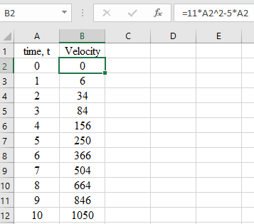
Use the Excel to find the velocity at a different time.
For the range of
Open the Excel and substitute the respective time. Apply the formula in column B.
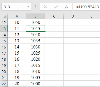
For the range of
Open the Excel and substitute the respective time. Apply the formula in column B.
For the range of
Open the Excel and substitute the respective time. Apply the formula in column B.
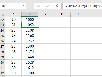
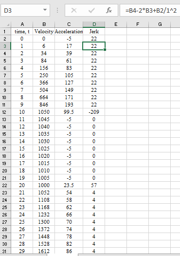
Thus, the velocity at every time is,
| time, t | Velocity |
| 0 | 0 |
| 1 | 6 |
| 2 | 34 |
| 3 | 84 |
| 4 | 156 |
| 5 | 250 |
| 6 | 366 |
| 7 | 504 |
| 8 | 664 |
| 9 | 846 |
| 10 | 1050 |
| 11 | 1045 |
| 12 | 1040 |
| 13 | 1035 |
| 14 | 1030 |
| 15 | 1025 |
| 16 | 1020 |
| 17 | 1015 |
| 18 | 1010 |
| 19 | 1005 |
| 20 | 1000 |
| 21 | 1052 |
| 22 | 1108 |
| 23 | 1168 |
| 24 | 1232 |
| 25 | 1300 |
| 26 | 1372 |
| 27 | 1448 |
| 28 | 1528 |
| 29 | 1612 |
| 30 | 1700 |
Recall the expression for the distance,
The expression for the distance is,
Use Simpson’s 1/3 rule tointegrate the above data.
Recall the expression for Simpson’s 1/3 rule.
Take the integral for the even space time,
Substitute all the value from the above table.
Solve further,
Solve further,
The total integral is equal to the sum of all individual integral.
Thus, the vertical distance travelled by the rocket is
Calculate the acceleration by numerical difference of the velocity.
Use the first derivative forward difference formula.
Substitute all the value from the time velocity table.
Calculate the acceleration for time
Substitute all the value from the time velocity table.
Similarly calculate all the value by using the Excel.
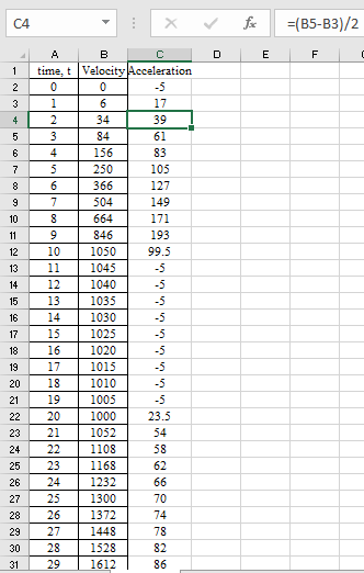
Use the first derivative backward difference formula to calculate acceleration for
Recall the first derivative backward difference formula.
Solve for
The below plot shows the relation between the Acceleration and time.
Write the expression for the Jerk.
Calculate the jerk by using the second order finite difference formula.
Write the second derivative forward difference formula.
Substitute all the value from the time velocity table.
Calculate the jerk for time
Substitute all the value from the time velocity table.
Similarly calculate all the value by using the Excel.
Use the second derivative backward difference formula to calculate acceleration for
Write the second derivative backward difference formula.
Solve for
The below plot shows the relation between the jerk and time.
Want to see more full solutions like this?
Chapter 24 Solutions
Numerical Methods for Engineers


- Kinetic energy of a fluid flow can be computed by 1 pv · vdV, where p(x, y, z) and v(x, y, z) are the pointwise fluid density and velocity, respectively. Fluid with uniform density flows in the domain bounded by x2 + z² = 6 and 0 < y<. = The velocity of parabolic flow in the given domain is v(x, y, z) 6 (6 – x² – 2²)j. Find the kinetic energy of the fluid flow.arrow_forward100 10 Circular disk Sphere 0.1 0.01 1 10 100 1,000 10,000 100,000 1,000,000 10,000,000 Reynolds number Re = U d/v A spherical weather balloon of 2 m diameter is filled with hydrogen. The total mass of the balloon skin and the instruments it carries is 3.7 kg. At a certain altitude the density of air is 1.0 kg/m3 and is 10 times the density of hydrogen in the balloon; the viscosity of air is 1.8x10⁻⁵ Ns/m3. Determine the steady upward velocity of the balloon. m/s Drag coefficlent Caarrow_forwardA closed thermodynamic system consists of a fixed amount of substance (i.e. mass) in which no substance can flow across the boundary, but energy can. For a closed themodynamic system we cannot add energy to the system, via substance (E ) (1.e. matter which contains energy is not allowed across the boundary) Across the Boundaries E° = No Q = = Yes W mass NO CLOSED = Yes SY STEM m = constant | energy YES Figure 1.1. If the substance inside the thermodynamic system shown in figure 1.1. (i.e. piston cylinder device) is air, is the system a Fixed closed system Moveable closed system A. В.arrow_forward
- Solve the following application problem: The model s(t) = -16?2 + 5? + 3 describes the height(in feet) of a diver at time ? is measured in seconds. Find the velocity of the diver when the diver hits the water.arrow_forwardTo be able to solve rectilinear problems with variable functions. Let A=1/V feet per second per second; V0= 5fps. Find A, V and t when s = 25 ft.arrow_forwardUse of Infinite Sequences and Series in Problem Solving of Special Theory of Relativity. A spacecraft travels fast the earth has a greater velocity (ⱱ) which approximates the speed of light. The time (to) measured in the spacecraft is different from the time (t) measured on earth. The time difference is given, to = t √1- ⱱ 2/c2 = t (1 – ⱱ 2/c2)1/2.arrow_forward
- Q16. A 3.4-kip car speeds up uniformly from 0 to 57 mph in 39 seconds up the 15⁰ incline. If the engine has an efficiency of e = 0.73, what is the power input (in hp) when the car's speed reaches that final speed? (1 hp = 550 ft-lb/s) Please pay attention: the numbers may change since they are randomized. Your answer must include 1 place after the decimal point. Take g = 32.2 ft/s². Your Answer: Answer 15°arrow_forwardThe displacement of a particle is given by s = 4t3 - 54t2 + 105t - 49 where s is in feet and t is in seconds. Plot the displacement, velocity, and acceleration as functions of time for the first 10 seconds of motion. After you have made the plots, answer the questions. Questions: Att- 2 sec, ft. v= ft/sec, a = ft/sec? %3D Att = 4.1 i ft. v= i ft/sec, a = i ft/sec? sec, Att = 8.7 i ft, v= i ft/sec, a = i ft/sec? sec, The velocity is zero when t = i sec and whent%3D i secarrow_forwardTo be able to solve rectilinear problems with variable functions. Let A = -t feet per second per second; V0 = 800 feet per second. How long a time will be required for the particle to come to rest, and how far will it travel in that time?arrow_forward
- From the image below, and using the given datum, match the variable expressions to their position coordinates, SA, SB and SC, where s A is for block A, $3 is for pulley B, and so is for pulley C. If an expression does not match any position coordinate, then match it to the "None" option. 1.k-q 2.0 3.p 4. k SA Datum bc SC k ✓ None SB ФВ A Р ⒸOFarrow_forwardQ6 The relationship between the velocity, u, of a construction vehicle (in km/h) and the distance, d (in metre), required to bring it to a complete stop is known to be of the form d = au² + bu + c, where a, b, and c are constants. Use the following data to determine the values of a, b, and c when: a) u 20 and d = 40 b) u = 55, and d = 206.25 c) u = 65 and d = 276.25 [Note: Use an appropriate standard engineering software such as MATLAB, CAS calculator, programmable calculator, Excel software]arrow_forward1) Is it possible to prescribe the velocity v0, so that the pendulum keeps rotating with alpha = pi/2 Explain clearly why? Given: L, g, and m. 2) After transient motion, the pendulum settles at steady state rotation atalpha = pi/3. Find the initial velocity v0. Given: L, g, m, sin(pi/3) = (squareroot(3)/2), cos(pi/3) = (1/2). [Hint: Use the conservation of energy and the 2nd Newton’s law.]arrow_forward
 Elements Of ElectromagneticsMechanical EngineeringISBN:9780190698614Author:Sadiku, Matthew N. O.Publisher:Oxford University Press
 Mechanics of Materials (10th Edition)Mechanical EngineeringISBN:9780134319650Author:Russell C. HibbelerPublisher:PEARSON
 Thermodynamics: An Engineering ApproachMechanical EngineeringISBN:9781259822674Author:Yunus A. Cengel Dr., Michael A. BolesPublisher:McGraw-Hill Education
 Control Systems EngineeringMechanical EngineeringISBN:9781118170519Author:Norman S. NisePublisher:WILEY
 Mechanics of Materials (MindTap Course List)Mechanical EngineeringISBN:9781337093347Author:Barry J. Goodno, James M. GerePublisher:Cengage Learning
 Engineering Mechanics: StaticsMechanical EngineeringISBN:9781118807330Author:James L. Meriam, L. G. Kraige, J. N. BoltonPublisher:WILEY